I’ve developed an approach for position sizing that allows for conviction-adjusted sizing based on a quantitative measure of statistical significance.

I previously exclusively used volatility-adjusted sizing, which is an approach that attempts to keep a standard deviation move (in dollars) in any one position equal across all positions.

I still believe in that approach when diversifying across equal-conviction trades, but when you’re trading based on quantifiable statistical outcomes it becomes logically inconsistent with your results. I’ll describe that approach first.

Volatility-adjusted Positioning

Suppose you want to size your positions in a “volatility equalized” manner. In other words, irrespective of your trade thesis, you want the expected random fluctuations in any one position to be about the same value in dollars.

Last Price per Share
QQQ = $396.92
XLI = $103.92
XLF =  $38.82

To do this you’d first compute the volatility for each security however you like. Some would use implied volatility, I would use a 28 trading day realized volatility. Perhaps you’d want to use a forecast. Annualized, daily, or weekly doesn’t matter, as it’ll cancel out in the end.

1 Week Realized Volatility (over 52 weeks)
QQQ = 2.22%
XLI = 1.89%
XLF = 2.42%

Next, you’d multiply that value against the current trading price of each security. I call the resulting value the “standard move” - it’s a dollar amount that you should expect to see your PnL swing per share/contract with some regularity¹.

Standard Move per Share per Week
QQQ = $8.81
XLI = $1.96
XLF = $0.94

I call the security with the greatest price the controlling leg. Its base position size is 1. I then set the positions of the other legs by dividing the standard move of the controlling leg by the standard move of each position. This gives us the position ratios we need for our portfolio. We just need to multiply this set of numbers by a constant until we get the total amount we’re looking to invest.

QQQ = 1.00 (controlling leg)
XLI = 4.50
XLF = 9.37

Minimum portfolio cost (fractional shares) = $1,228.30
Target investment = $10,000.00
Required multiple = 8.14

Final position sizing:
QQQ =  8.1
XLI = 36.6
XLF = 76.3

Fractional shares are possible these days but I usually just find a multiple that is a compromise between total investment and minimal “error”.

Conviction-adjusted Positioning

If your statistical results for one trade are twice as “strong” versus another trade it would be absurd for those positions to have equal size. Even more absurd would be to give a significant allocation to a position that is based on a signal that may have zero effect.

I needed a way to take my statistical results and turn them into rational allocations.

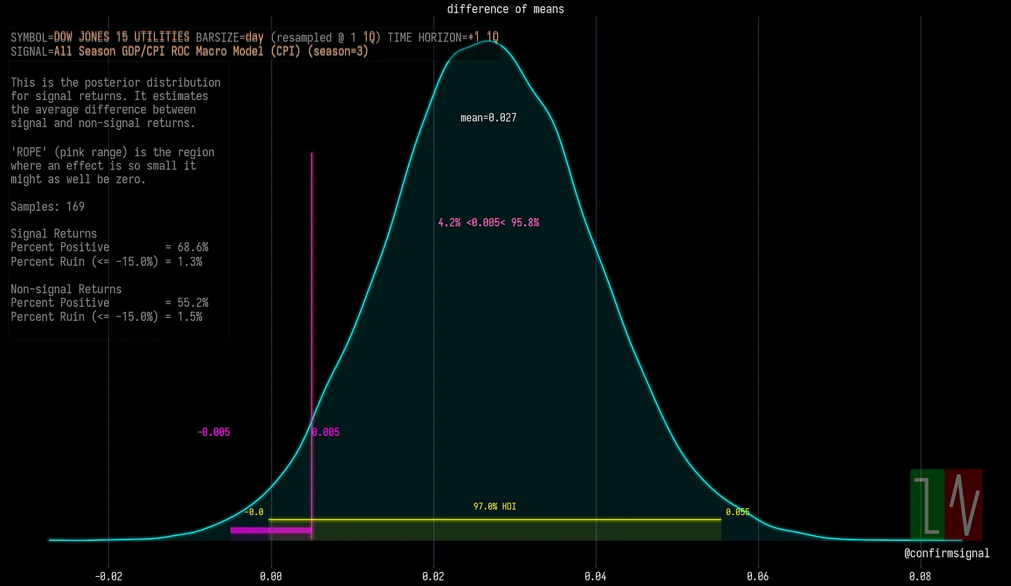
The above posterior difference of means result summarizes the statistical significance of a signal. This is the information I want to encode in my conviction-based positioning.

First, I had to figure out what pieces of this result I needed to include in my significance metric. The high density interval (HDI, aka credible interval) is a clear choice for focus. The ROPE and its relation to the HDI is also something I want to consider. I like the percent positive metric, but since we’re using the HDI so far I’ll focus on the HDI’s mean value instead.

Having selected the important components, I had to figure out how this significance metric should behave. I want a larger HDI mean to cause a greater significance. I want to punish results that have overlap around the ROPE based on the amount of their overlap. I also want to punish results that have an HDI that extends below (to the left) of the ROPE; I don’t want significant probablity mass to exist around negative returns.

I played around in Excel and my black board for a bit until I had something that behaved in a logically consistent manner (in my subjective opinion), and here’s what I ended up with. I should note that this is applied to my difference of means posterior exclusively.

We start with the mean difference of means. This is the foundation of the metric. The greater the difference of means is on average, the better the score.

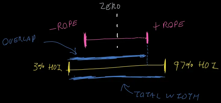
Next, we want to punish ambiguity. This means punishing a score that has a significant probability mass around and below the ROPE. If there is no overlap, there should be no punishment.

To compute this punishment ratio I found the depth of overlap, including the amount that the HDI descends below the ROPE. I then divide it by the total width of the HDI, and subtract this ratio from one. This result times the mean difference of means is the score.

I then compute the total of this value across all of my positions, and each security is sized according to its share relative to that total.

 Security | Significance Metric | Position Share
----------|---------------------|------------------------
 VPU      |  2.70e-2            | 2.70e-2 / 0.054 = 50%
 EDV      |  2.44e-3            | 2.44e-3 / 0.054 = 5%
 GLD      |  2.49e-2            | 2.49e-2 / 0.054 = 45%

I originally sized these positions based on the above volatility measure, which has them all between 28 and 40%. This means I had a low conviction position with far more capital allocated to it than is justified, which is the logical inconsistency I warned about earlier.

This approach likely has flaws I have not considered, and it is not the only way I could have developed this fitness metric for position sizing. However I think this is a huge step forward in rational position sizing for my own purposes.

Conclusion

Neither approach protects us from oversized drawdowns. That’s up to you when you allocate how much money you’re willing to lose. The idea with the conviction allocation is to reward high-conviction trades with more capital and punish low-conviction trades with less. The idea with the volatility approach is to attempt to even out the random fluctuations in your positions.

Footnotes